
Precise trigger control with DISB electronics

Introduction
In spectroscopy, the exact timing of when a measurement begins can be critical and, this timing is controlled through the spectrometer’s electronical interface. Therefore, it is important to understand how the spectrometer’s electronics handles trigger signals and exposure timing to ensure that measurements start at the intended moment and that signal integration occurs only during the defined integration period.
In general, three measurement scenarios can be identified:
- The spectrum is stable and time-insensitive
- The spectrum is present only for a limited duration at specific times
- The spectrum changes as a function of time
For stable, time‑insensitive signals, the exact start time of spectral acquisition is generally not critical. In such cases, the integration time is simply chosen to maximize signal strength, and precise trigger control becomes largely irrelevant. Even when the spectrum evolves slowly over time – as in UV‑VIS absorption during chromatographic separation – the changes can be followed by continuously acquiring short measurements, and precise timing control is likewise unnecessary.
However, when the spectrum is available only for a limited duration or at specific intervals, precise control over the measurement start time becomes essential. Without accurate timing, it may be difficult, or even impossible, to capture a meaningful signal.
In such situations, the spectrometer’s electronics must provide both precise triggering capabilities and flexibility in how triggers are controlled, including their source and timing. This is particularly important in applications involving moving samples (e.g., objects on a conveyor belt, flow in a pipe, or scanning systems) or systems that rely on pulsed light sources such as lasers or flash lamps.
In other cases, the spectrum itself changes rapidly over time, making accurate control of the integration period equally important. A classic example is Laser-Induced Breakdown Spectroscopy (LIBS), where both the start and end of the measurement must be carefully controlled. The emission spectrum from the decaying plasma evolves rapidly on timescales ranging from nanoseconds to milliseconds.
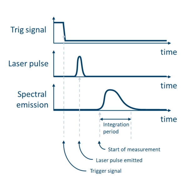
Figure 1 – Example of timing control in LIBS measurements. The laser pulse is emitted after a defined delay from the trigger signal, and the spectrum is recorded after an additional delay for a specified integration time.
For systems using pulsed light sources, such as xenon flash lamps, the duration of the light pulse effectively defines the useful integration window. Even in these cases, precise control of the spectrometer’s integration timing helps ensure that signal is collected only while the lamp is emitting, thereby reducing unwanted noise contributions, such as dark current.
In the following chapters, we will explore the triggering options available in the Ibsen Photonics Digital Image Sensor Board (DISB) electronics, along with key timing considerations and methods for synchronizing measurements with external light sources. It is important to note that the specific detector array used in a spectrometer strongly influences the achievable precision in controlling the start and end of the integration period.
Typical measurement setups
In spectroscopic measurements, the timing relationship between the spectrometer, the light source, and any external control system is defined through trigger signals and a set of fixed and variable delays. A trigger signal is typically an electrical signal – most commonly a transition between voltage levels, often defined by TTL logic between 0V and 3.3V or 5V – that instructs a device to perform a specific action, such as initiating an exposure or emitting a light pulse. Depending on the system, the trigger may be defined by either a rising edge (low-to-high transition) or a falling edge (high-to-low transition), and the selected trigger polarity must be consistent across all connected devices to ensure proper synchronization.
Trigger signals can originate from different sources depending on the measurement setup. They may be generated by an external controller (e.g., a timing unit or data acquisition system), by the spectrometer itself, or by the light source if it provides a trigger output. In many practical systems, a single master trigger signal is distributed to multiple components to ensure synchronization.
When a trigger signal is used to control a pulsed light source, the emission of the light pulse usually occurs after a defined delay relative to the trigger event. Similarly, the spectrometer has an inherent delay and can furthermore be configured to start its integration after an additional programmable delay. These delays are critical parameters, as they determine the temporal overlap between the light emission and the spectrometer’s integration window.
To ensure correct and reproducible measurements, the trigger signals supplied to both the spectrometer and the light source must be properly synchronized. This is often achieved by using a shared trigger source or by distributing a common timing signal to all relevant devices. In more advanced setups, a Digital Delay Generator (DDG) can be introduced to precisely control the relative timing between multiple trigger signals, allowing independent adjustment of delays for the spectrometer and the light source with high temporal resolution.
In addition to the start of integration, the timing of the readout process is also an important consideration. In most spectrometer systems, the detector is read out only after the integration period has completed. The readout time therefore introduces a fundamental limit on how frequently consecutive measurements can be acquired. For high-speed or time-resolved applications, this constraint must be considered when designing the overall timing scheme.
For certain applications, more advanced measurement techniques such as lock-in detection may be employed. In lock-in measurements, the signal of interest is modulated at a known frequency, and the spectrometer is synchronized with this modulation. By selectively measuring signals that are phase-locked to the modulation frequency, it is possible to significantly improve the signal-to-noise ratio and suppress background contributions.
Understanding these fundamental timing relationships is essential for configuring a spectrometer system correctly, particularly in applications involving pulsed sources, transient phenomena, or high-speed measurements.
Trigger options for DISB electronics
In many cases the need for an external DDG can be eliminated when using DISB electronics. The DISB system is capable of generating programmable delays internally, while also accepting external trigger inputs and providing trigger output signals (AUX0). This flexibility and control enable the spectrometer to both synchronize with external devices and actively control them – such as triggering a light source or a shutter – within a single, integrated timing framework.
All DISB spectrometer electronics support three different trigger options.
- Software / SPI trigger
- External hardware trigger input
- Internal trigger generator
Via the DISB’s registers it is possible to enable or disable any or all of the triggers to best suit the need of a given application.
The software trigger initiates a measurement when a specific software command is transmitted directly to the DISB electronics’ SENSOR CTRL register. This command can be transmitted via SPI (Serial Peripheral Interface – a direct interface to the DISB electronics) or over USB when using the DISB-USB bridge.
Because this trigger method depends on the timing of command execution in your microcontroller and on the communication‑interface transfer latency, the precision of the measurement start is limited – typically to the millisecond range. This trigger mode is well suited for applications where sub‑millisecond timing accuracy is not required, or in systems where the DISB electronics controls the light source (see Chapter 4.2.).
Adding to this, the DISB electronics is equipped with two external hardware trigger inputs (EXT_TRIG1 and EXT_TRIG2) accepting voltage levels of 3.3V or 5V activating on the falling edge of the trigger signal, this allows for great flexibility in the system as the electronics can accept trigger input from multiple source and even using different TTL logic.
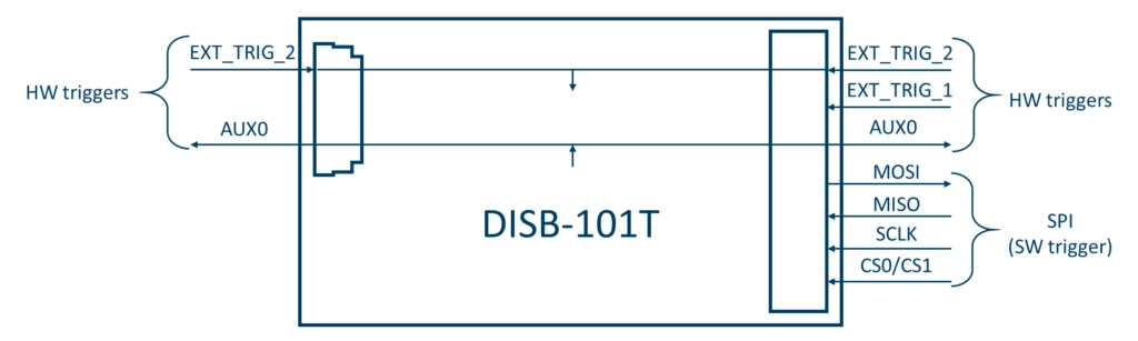
Figure 2 – Connectors for HW and SW triggers on DISB-101T electronics. The AUX0 and EXT_TRIGGER_2 is electrically connected to an external connector as well as the SPI-connector.
The delay between receiving the trigger and starting the measurement can be adjusted in increments of 200 ns. This method provides the most accurate control of the start of the integration period and can – depending on what the detector supports – lead to sub-microsecond accuracy.
The internal trigger generator enables the DISB electronics to autonomously produce periodic trigger pulses. This functionality is particularly useful in measurement setups where the DISB electronics serves as the central controller, coordinating the timing of all connected devices. In such configurations, the Auxiliary Lamp Control output (AUX0) can be used to distribute trigger signals to external components, such as a light source or a mechanical shutter.
One example is the acquisition of multiple spectra using a detector that exhibits a delay between receiving a trigger signal and the actual start of integration. In this case, a programmable delay can be introduced between the internal trigger and the AUX0 output, ensuring that the light source is activated only when the detector is ready to acquire data.
Another application is lock-in spectroscopy, where the internal trigger defines the measurement frequency while the AUX0 output controls the modulation of the light source, either directly or via a chopper or shutter mechanism. This enables synchronized, alternating measurements of the reference and the sample signal.
The timing parameters of the internal trigger system are configurable with high precision. The interval between trigger pulses can be adjusted in increments of 50 µs, while the delay between the trigger event and either the AUX0 output or the start of detector integration can be set with a resolution of 200 ns.
Timing consideration using the external hardware trigger
As standard most DISB electronics operates on 5 MHz clock frequency, which allows for adjusting the trigger time delay in 200 ns increments. When adjusting the timing delay of the external trigger, it is necessary to account for all delays inherent to the detector and/or electronics in order to properly synchronize the start time of the detector integration with sample measurement.
Common delays include the electronics propagation delay (Td), i.e. the time it takes for a trigger signal to “travel” through the electronics and be registered by the FPGA, inherent detector start time or dummy scan read outs.
When these values are known and more importantly precisely defined with very low variation, known as jitter, achieving accurate timing becomes fairly straightforward.
Examples of inherent trigger delays
A practical example of this can be seen with the DISB-101T electronics, which are built around Hamamatsu Photonics’ S11639N-01 CMOS detector and offer an impressively low jitter of just 10 ns.
The DISB-101T board introduces a propagation delay of 500 ns. In addition, the detector requires 3.5 clock cycles from receiving a Sensor Start pulse to the point where it begins actively measuring. At a clock frequency of 5 MHz, 3.5 clock cycles correspond to 700 ns. Combined with the 500 ns propagation delay, this results in a total delay of 1200 ns from the moment a trigger signal is received to when the detector starts integrating the signal.
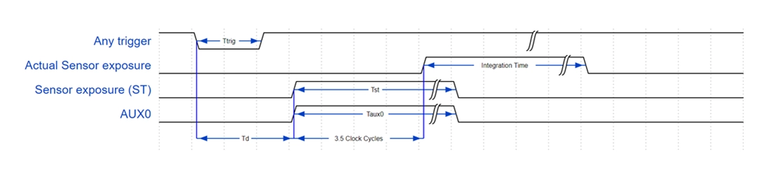
Figure 3 – Timing delay inherent to DISB-101T and Hamamatsu’s S11639 CMOS detector
This total delay must be taken into account when configuring the system. For example, if a delay of 10 µs from receiving a trigger input to the start of measurement is required, the inherent 1.2 µs delay (from propagation and detector response) must be subtracted. In this case, the DISB delay setting should be configured to 8.8 µs (10 µs – 1.2 µs) to achieve the desired timing.
| Electronics | Detector(*) | Propagation Delay | Detector delay | Dummy readout | Jitter | Combined delay |
|---|---|---|---|---|---|---|
| DISB-101T | S11639 S13496 | 500 ns | 3.5 clk (700 ns) | No | 10 ns | 1200 ns |
| DISB-105 | S14739 | 500 ns | 3.5 clk (700 ns) | No | 10 ns | 1200 ns |
| DISB-220 | S838x | 150 ns | 0 ns | Yes | 20 ns | Detector specific |
| DISB-290 | S838x | 150 ns | 0 ns | Yes | 20 ns | Detector specific |
| DISB-315 | S10420 | 200 ns | 0 ns | Yes | 20 ns | Detector specific |
| DISB-380 | S11156 | 360 ns | 0 ns | No | 10 ns | 360 ns |
| DISB-386 | S11850 | 200 ns | 0 ns | Yes | 20 ns | Detector specific |
| DISB-400 | G13913 | 1040 ns | 1.5 clk (1500 ns) | No | 20 ns | 2540 ns |
| DISB-411 | G11620 | 500 ns | 0 ns | No | 10 ns | 500 ns |
| DISB-466 | G11508 G1147x | 430 ns | 5.5 clk (1100 ns) | No | 10 ns | 1530 ns |
| DISB-486 | G17225 | 430 ns | 42.5 clk (16.9 µs) | No | 110 ns | 17.33 µs |
(*) The DISB electronics can handle multiple detectors from same detector family, i.e., number of pixels, pixel height, NIR enhancement, etc.
Controlling a light source from the DISB
The DISB electronics can be configured as the system’s master controller by sending trigger signals to other components such as light sources or shutters. In this configuration, the DISB outputs a trigger signal on the AUX0 pin (Auxiliary Lamp Control) with a precisely defined timing relationship relative to the start of the integration period.
For example, the DISB-101T electronics have an inherent delay of approximately 1200 ns, consisting of a 500 ns propagation delay and a detector start time of 3.5 clock cycles. By applying an equivalent delay to the AUX0 output signal, the activation of a lamp or laser can be synchronized precisely with the moment the detector begins its active measurement. This approach also allows compensation for any additional delay introduced by the light source itself.
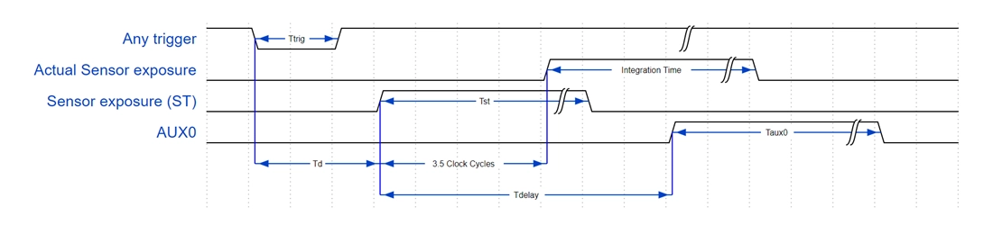
Figure 4 – Time diagram showing how the AUX0 output signal can be set to trigger after a measurement is started
Examples of precise trigger control
There are many situations where accurate triggering is essential to achieving consistent, high-quality measurements. A classic example is Laser-Induced Breakdown Spectroscopy (LIBS), where the signal typically is defined in three stages
- Early continuum (electron-ion plasma) ~0-200 ns
- Atomic/Ionic emission ~200 ns to 10-20 µs
- Molecular emission ~20 µs to milliseconds
For most application only the Atomic/Ionic emission is of interest which means that even a shift of a few microseconds in the measurement’s timing can have a dramatic impact. Poor timing may result in the signal being overwhelmed by the laser pulse itself, while excessive delay can mean missing the emission entirely.
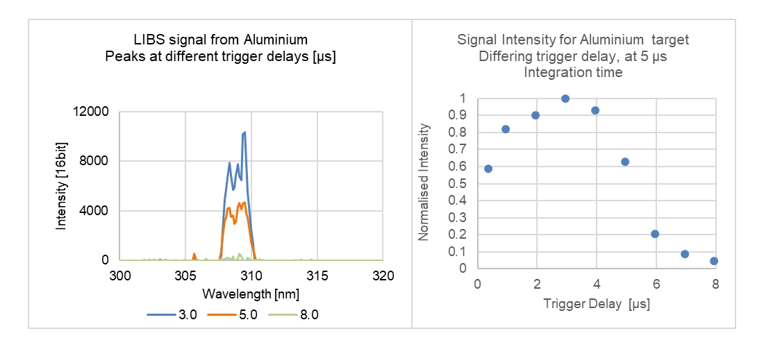
Figure 5 – Intensity of Aluminium’s LIBS signal of as a function of time delay.
Another highly relevant example involves xenon flash lamps, which are commonly used in UV–VIS applications due to their broad spectral emission. These lamps generate light by ionizing xenon gas, producing a short-lived discharge pulse.
Because the emitted light exists only for a brief duration – often as a single pulse or a series of pulses – accurate control of the spectrometer trigger is essential. Proper timing ensures that the measurement is captured during the emission period, maximizing signal quality and avoiding unnecessary noise.
Want to know more?
For further information see below.